When Is Simple Randomisation Enough?

Simulations

To determine how big a problem group imbalance is for different sample sizes, I’m going to simulate randomly allocating participants to one of two experimental groups 1000 times for different total sample sizes, and find out how often group imbalance occurs.

First, I create a function that randomly allocates participants to groups, and finds the percentage of participants that were assigned to the first of the two groups.

randomise_group_prop <- function(total_ppts, num_groups) {
  
  allocation <- randomise(total_ppts, num_groups)

  in_class <- sum(allocation[allocation == 1])

  (in_class / total_ppts)*100

}

Next, I use R’s replicate() function to randomly assign participants to groups multiple times.

Here, I’ve chosen to run the function 1000 times for each sample size.

First, let’s look at what happens when we run simple randomisation 1000 times with a total participant number of 20.

set.seed(901)
small_sample_results <- replicate(n = 1000, randomise_group_prop(20, 2))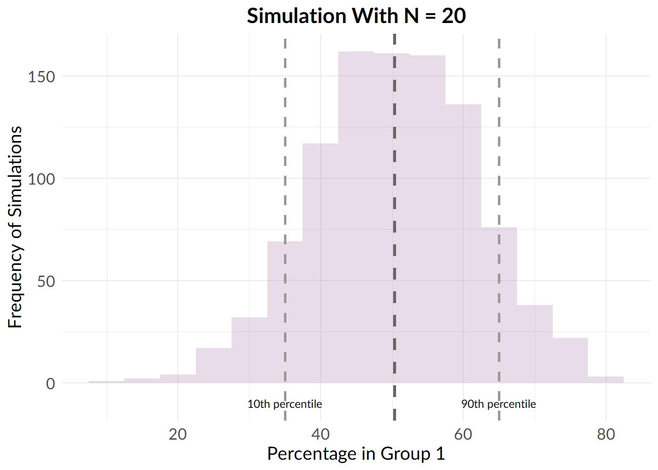

From this plot, we see that on average, we wind up with a roughly equal number of participants in each group, but, there are a lot of samples with large group imbalance.

Next, let’s see what happens if we increase the sample size to 100 participants.

set.seed(81)
medium_sample_results <- replicate(n = 1000, randomise_group_prop(100, 2))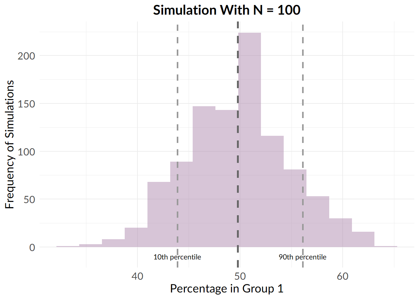

Now, the spread is smaller, but, we still see a substantial proportion of samples where the groups are imbalanced.

Next, let’s increase the sample size to 1000.

set.seed(9001)
large_sample_results <- replicate(n = 1000, randomise_group_prop(1000, 2))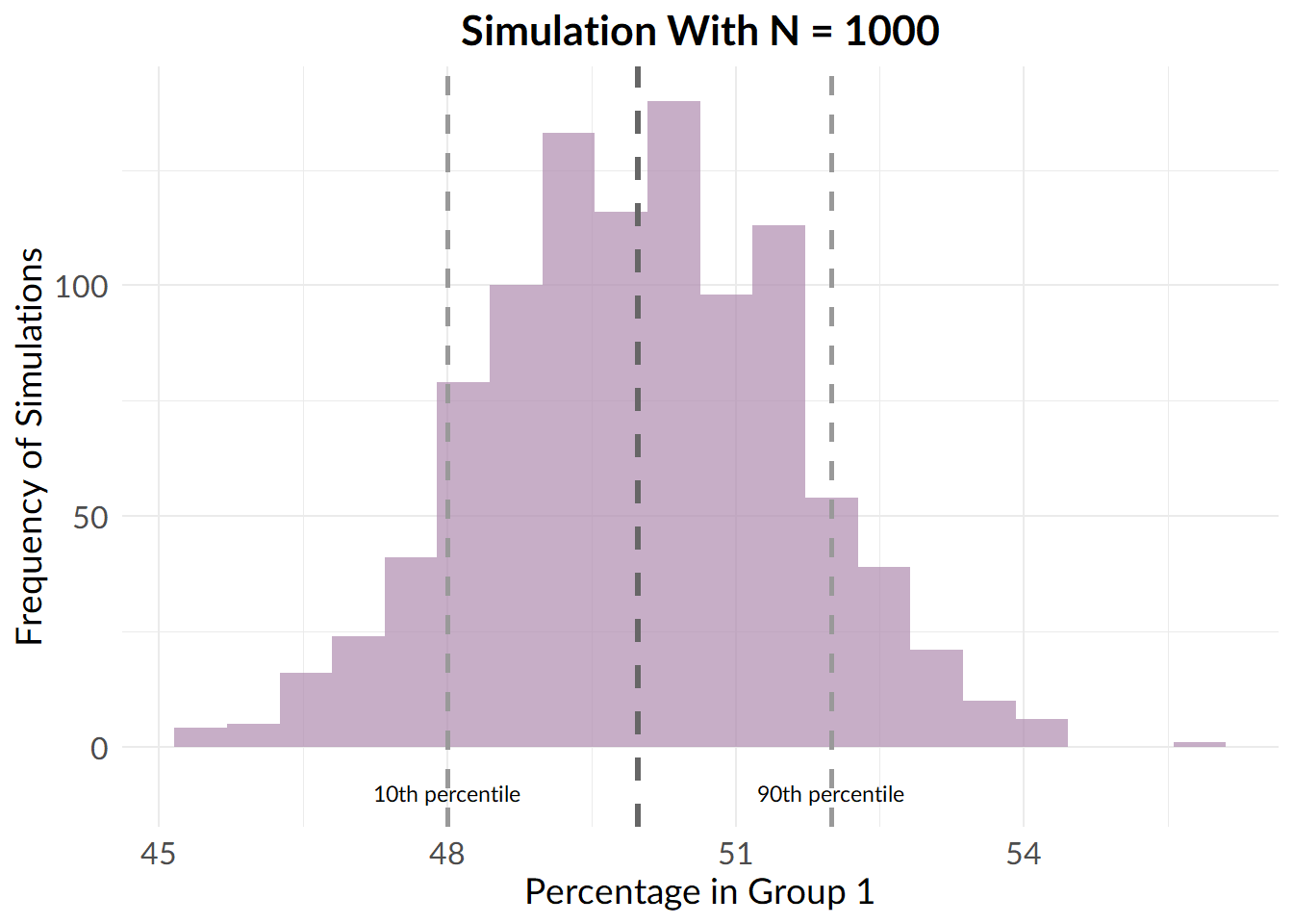

Finally, we increase the sample size to 10000 participants.

set.seed(8976)
larger_sample_results <- replicate(n = 1000, randomise_group_prop(10000, 2))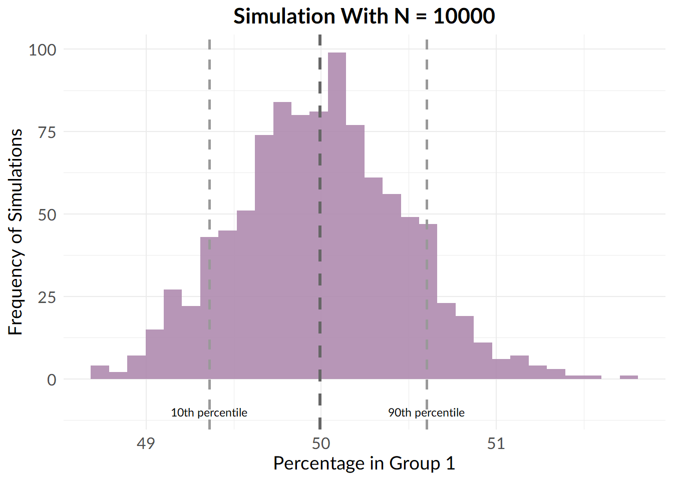

Beautiful.

So, what does these simulations tell us?

Well, when we have a sample size of around 100 participants, we frequently obtain imbalanced groups. For instance, in 10% of my simulations, I wound up with 35% or fewer participants allocated to group 1.

By the time we get to 1000 participants, things are looking much better, and by 10000 participants, the problem has basically gone away.

(Note that I’ve used a simple experimental design with two experimental groups. With a more complicated experimental design, we’d expect to need a larger sample size before group imbalance stopped being a problem.)

Interpretation

So, does this mean that simple randomisation a bad choice when your sample size is in the ~100-500 participant range?

Fundamentally, it depends on how worried you are about the impacts of group imbalance on your experiment.

Broadly, there are two major reasons why group imbalance can be a problem:

1. Loss of statistical power
2. Confounding variables

The first problem with group imbalance is that it reduces the statistical power to detect significant effects. This is a problem if you’re anticipating a small or medium effect size, but less so if you’re anticipating a large effect size.

The second problem with group imbalance is a somewhat trickier one to deal with. When groups are imbalanced, participant characteristics (for instance, the demographics of the participants) can wind up being split unevenly across the experimental groups. This can introduce confounding variables into the experiment.

For instance, let’s say you’re running an educational intervention to improve the maths ability of your students. You have a treatment group who receive the intervention, and a control group who are taught as normal. At baseline, you notice that a small subset students are already performing much better than the others. If these students are all assigned to the intervention group, this will cause the intervention to look more effective than it really is. Likewise, if these students are all assigned to the control group, the intervention will appear less effective than it really is.

Now, randomisation should mean that these students are split roughly evenly across the two expeirmental groups. However, group imbalance makes it more likely that the high ability students are not spread evenly across the two groups, introducing a potential bias into the results.

Unfortunately, this issue is a particularly tricky one, because it’s hard to be sure how much it may have affected the experiment. Once the experiment has ended and we know how participants were allocated, we can check whether or not potentially confounding variables were spread evenly across the experimental groups. But, we likely won’t have measured all of the possible confounding variables, and we can only know about the variables that we do measure.

If Not Simple Randomisation, What Else?

Alternatives to simple randomisation include, but are not limited to:

• blocked randomisation: participants are randomly assigned within ‘blocks’ such that an equal number of participants are assigned to each group within the block.
• stratified randomisation: participants are randomly assigned to groups in such a way as to ensure that certain variables are spread out equally across groups.

For instance, here’s a function I made to implement block randomisation:

block_randomise <- function(total_ppts, num_groups, block_size) {
  
  if(block_size %% num_groups > 0) {
    warning("Your block size should be a multiple of the number of experimental groups")
  }
  
  else {
    
    total_blocks <- ceiling(total_ppts / block_size)
    
    groups <- c(1:num_groups)
    
    group_reps <- block_size / num_groups
    
    block <- rep(groups, group_reps)
    
    unlist(replicate(n = total_blocks,
            sample(block, length(block), replace = FALSE),
            simplify = FALSE))
  }
}

table(block_randomise(90, 3, 9))

## 
##  1  2  3 
## 30 30 30

As with all options in experimental design, these randomisation strategies also have their own strengths and weaknesses. For instance, one issue with blocked randomisation is that if the blocks are all of equal size, and the investigator becomes unblind to the allocation status of a participant, it can become possible for them to predict the allocation of subsequent participants.²

A/B Testing In The World of Tech

When sample sizes are small, you’re probably better off avoiding simpe randomisation. But, what about in the world of tech and A/B testing? Should we be avoiding simple randomisation?

Well… here it feels a bit more of a toss up. On the one hand, sample sizes in tech tend to be larger, meaning that the probability of group imbalance is much smaller. It’s also by far the simplest method of randomisation available.

That being said, downsides of blocked randomisation tend to revolve around the added risk of investigator bias - which is typically less of a problem in tech setting since the intervention is carried out by a computer. So, I’d say it usually doesn’t hurt to implement a slightly more complicated randomisation method.

In my opinion, though, the most important thing is to be making an informed choice; think about what randomisation methods are available, their respective strengths and weaknesses, and decide which is the most suitable for your study. Don’t just let some A/B testing software take the decision entirely out of your hands.