Why Linear Regression Estimates the Conditional Mean
Because you can never know too much about linear regression.
Introduction
If you look at any textbook on linear regression, you will find that it says the following:
“Linear regression estimates the conditional mean of the response variable.”
This means that, for a given value of the predictor variable \(X\), linear regression will give you the mean value of the response variable \(Y\).
Now, in and of itself, it’s a pretty neat fact… but, why is it true?
Like me, you may have been tempted to take to google for an answer. And, like me, you may have found the online explanations hard to follow.
This is my attempt to break down the explanation more simply.
Recap on Linear Regression
Let’s begin with a quick recap on linear regression.
In (simple) linear regression, we are looking for a line of best fit to model the relationship between our predictor, \(X\) and our response variable \(Y\).
The line of best fit takes the form of an equation
\[Y = \beta_{0} + \beta_{1}X\]
where \(\beta_{0}\) is the intercept, and \(\beta_{1}\) is the coefficient of the slope.
To find the intercept and slope coefficients of the line of best fit, linear regression uses the least squares method, which seeks to minimise the sum of squared deviations between the \(n\) observed data points \(y_{1}...y_{n}\) and the predicted values, which we’ll call \(\hat{y}\):
\[\sum_{i=1}^{n} (y_{i} - \hat{y})^2\]
And, as it turns out, the values for the coefficients that we obtain by minimising the sum of squared deviations always result in a line of best fit that estimates the conditional mean of the response variable \(Y\).
Why? Well, the “simple” answer is that it can be proved mathematically. That’s not a very satisfying or helpful answer though.
However, one thing I do think is helpful for understanding the “why” is exploring the sum of squared deviations in a slightly simpler context.
The Sum of Squared Deviations Method
So far, we’ve talked about minimising the sum of squared deviations in the context of linear regression. But, minimising the sum of squared deviations is a general method that we can also apply in other contexts.
For instance, let’s generate a dataset of 1000 numbers, with a mean of ~20 and a standard deviation of 2.
set.seed(8825)
sample_data <- rnorm(1000, mean = 20, sd = 2)

# confirm mean is ~= 20
mean(sample_data)
## [1] 19.92143Now, we could calculate the sum of the squared deviations of each of these data points from the mean…
sum((sample_data - mean(sample_data))^2)## [1] 4004.373…(which is exactly what we’d need to do to calculate the standard deviation of the data)
And we could also calculate the sum of the squared deviations of these data points from any other value, such as the median, mode, or any other arbitrary value.
For instance, here’s the what we get if we calculate the sum of squared deviations of each data point from the median.
sum((sample_data - median(sample_data))^2)## [1] 4008.821So now, let’s calculate the sum of the squared deviations using a variety of different values:
# values to calculate the deviation from in our dataset
dev_values <- c(0, 5, 10, 12, 15, 18, 19, 19.92, 21, 22, 25, 28, 30, 35, 40)

# generate empty list
squared_residuals <- rep(NA, length(dev_values))

# calculate sum of squared deviations of the data from each value in dev_values
for (i in 1:length(dev_values)) {

  squared_residuals[i] = sum((sample_data - dev_values[i])^2)

}

squared_residuals
## [1] 400867.938 226653.590 102439.242 66753.502 28224.893 7696.285
## [7] 4853.415 4004.375 5167.676 8324.806 29796.197 69267.588
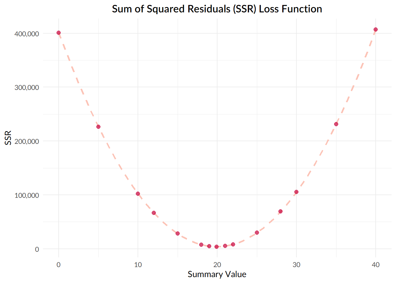
## [13] 105581.849 231367.501 407153.153Next, let’s plot the resulting sum of squared deviations obtained using each value:
data.frame(dev_values = dev_values, squared_residuals = squared_residuals) %>%
  ggplot(aes(dev_values, squared_residuals)) +
  stat_smooth(method="lm",
              formula = y ~ poly(x, 2),
              se = FALSE,
              colour = "#FCC3B6",
              linetype = "dashed") +
  geom_point(col = "#C70039", size = 2.2, alpha = 0.7) +
  labs(title = "Sum of Squared Residuals (SSR) Loss Function",
     x = "Summary Value",
     y = "SSR") +
  theme_minimal() +
  theme(text = element_text(family = "Lato"),
        plot.title = element_text(family = "Lato Semibold", hjust = 0.5)) +
  scale_y_continuous(labels = scales::comma)
Notice that the value that gives us the smallest sum of squared deviations, the lowest point on our curve, turns out to be 19.92, which is the mean of our dataset!
Now, this isn’t just a fun feature of our sample dataset; given any set of numbers \(x_{1}...x_{n}\), the value that results in the smallest sum of squared deviations will always be the mean.
And just in the same way, in linear regression, the predicted \(\hat{y}\) values that minimise the sum of squared deviations will always be the conditional mean of \(y\).
Now, this simulation might help you see how minimising the sum of squared deviations is equivalent to using the mean, but it still doesn’t explain why it’s the case.
For that, we need to look at the mathematical proof. Here, again, we’re going to focus on the slightly simpler use-case of minimising the sum of squares for a single set of values.
Mathematical Proof: Background
When we calculate the sum of squared deviations between some sample data \(y_{1}...y_{i}\), and another value \(\hat{y}\), what we’re really doing is passing the data through a function:
\[f(y) = \sum_{i=1}^{n} (y_{i} - \hat{y})^2\] And, in minimising the sum of squared deviations, our aim is to find the value for \(\hat{y}\) that minimises the output of the function.
Now, whenever we have a function whose output we want to minimise, we call the function a loss function, denoted as \(L(y)\).
So, we can write our sum of squared deviations function as this:
\[L(y) = \sum_{i=1}^{n} (y_{i} - \hat{y})^2\]
Whenever we want to find the value of \(\hat{y}\) that minimises a loss function, the way to solve this problem is by differentiation.
Why? Well, let’s take a look back at our plot, where we calculated the sum of squared deviations for different values of \(\hat{y}\).
The value that we want to find out, the one that minimises the sum of squared deviations, is the one at the lowest point of the curve, where the gradient of the curve is equal to zero.
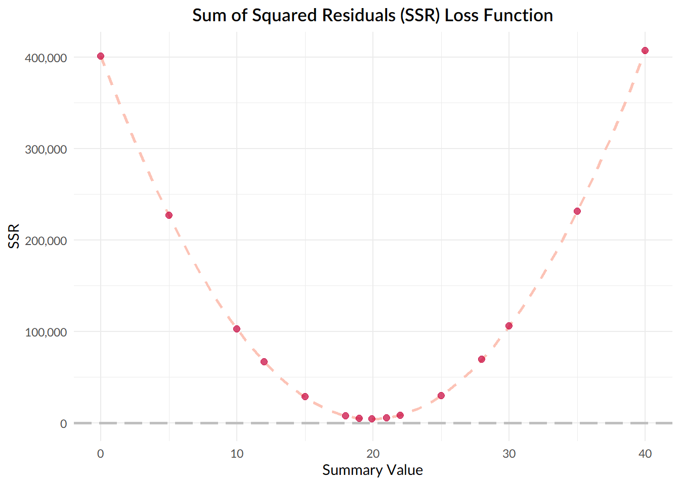
And so, what we’re really doing here is asking, what value does my summary statistic take, at the point at which the gradient of the sum of squared deviations function is equal to zero?
And finding gradients? Well, that’s a job for differentiation!
So, we want to differentiate our loss function:
\[\displaystyle \frac{d}{d\hat{y}} \lbrace{L(y)}\rbrace = \frac{d}{d\hat{y}} \lbrace\sum_{i=1}^{n} (y_{i} - \hat{y})^2\rbrace\] Differentiating the loss function gives us this:
\[\displaystyle \frac{dL}{d\hat{y}} = \sum_{i=1}^{n} -2(y_{i} - \hat{y})\] It can be a little tricky to understand what’s happened here, especially if you’re not using to differentiations involving \(\sum_{}\) symbols and \(y_{i}\) terms.
To make it a bit clearer what I’ve just done, I’m going to momentarily pause on differentiating our actual loss function and instead detour to a simpler problem, that of differentiating the equation \(y = (1 - \hat{y})^{2}\).
Now, we can write this equation like so:
\[\displaystyle y = (1 - \hat{y})(1 - \hat{y})\]
Which, expanded out, gives us the following:
\[\displaystyle y = (1 - 2\hat{y} + \hat{y}^{2})\]
Finally, differentiating the above gives us this:
\[\displaystyle \frac{dy}{d\hat{y}} = (2\hat{y} - 2)\] which is also equivalent to this:
\[\displaystyle \frac{dy}{d\hat{y}} = -2(1 - \hat{y})\] And, the differentiation works pretty much the same way for our actual function, \(L(y) = \sum_{i=1}^{n} (y_{i} - \hat{y})^2\):
\[\displaystyle \frac{dL}{d\hat{y}} = \sum_{i=1}^{n} -2(y_{i} - \hat{y})\]
Now, as mentioned earlier, to minimise the loss function, we need to find the value of \(\hat{y}\) when the gradient is zero, so let’s set this whole thing equal to zero:
\[\displaystyle 0 = \sum_{i=1}^{n} -2(y_{i} - \hat{y})\]
Divide both sides by -2 and we get this:
\[\displaystyle 0 = \sum_{i=1}^{n} (y_{i} - \hat{y})\]
Now, in the same way that \(3(5- 4)\) is the same as \(3 * 5 - 3 * 4\), the sum of \(y_{i} - \hat{y}\) is the same as saying the sum of the \(y_{i}\) values, minus the sum of adding up \(\hat{y}\) n times:
\[\displaystyle 0 = \sum_{i=1}^{n} y_{i} - \sum_{i=1}^{n}\hat{y}\]
And, the sum of adding up \(\hat{y}\) n times can also be written like so:
\[\displaystyle 0 = \sum_{i=1}^{n} y_{i} - n\hat{y}\]
We want to find the value of \(\hat{y}\), so let’s rearrange the equation a little:
\[\displaystyle n\hat{y} = \sum_{i=1}^{n} y_{i}\]
Finally, let’s divide both sides by n to find the value of \(\hat{y}\).
\[\displaystyle \hat{y} = \frac{\sum_{i=1}^{n} y_{i}}{n}\] And let’s look at what we’re left with here; \(\hat{y}\) is equal to the sum of all the \(y_{1}...y_{n}\) values in the data set, divided by \(n\), the number of values in the dataset… otherwise knows as, the mean of the \(y\) values!
And that’s that!